MLegS Tutorial 06: Vector Field Manipulation

Disclaimer: This MLegS tutorial assumes a Linux or other Unix-based environment that supports bash terminal commands. If you are using Windows, consider installing the Windows Subsystem for Linux (WSL).

In this tutorial, an effective approach for manipulating a divergence-free (solenoidal) vector field using the Toroidal-Poloidal (TP) decomposition is introduced. For an arbitrary vector field in a cylindrical coordinate system,

\[\mathbf{V} = V_r \hat{\mathbf{e}}_r + V_\phi \hat{\mathbf{e}}_\phi + V_z \hat{\mathbf{e}}_z,\]

it can be expressed as a set of three scalar components: \( V_r \), \( V_\phi \), and \( V_z \). However, directly using these components as state variables during simulations often leads to difficulties due to their coupling caused by physical constraints (e.g., incompressibility) or analyticity requirements (e.g., eliminating coordinate singularities at \( r = 0 \)).

MLegS provides subroutines for performing TP decomposition, including projecting a vector field into its toroidal and poloidal components and reconstructing the vector field from given toroidal and poloidal scalars. For a divergence-free vector field \( \mathbf{V} \), TP decomposition is:

\[\mathbf{V} = \nabla \times \left\{\psi \hat{\mathbf{e}}_z \right\} + \nabla \times \left[ \nabla \times \left\{ \chi \hat{\mathbf{e}}_z \right\} \right] .\]

One may find more mathematical details in Lee & Marcus (2023)¹. Using the toroidal and poloidal scalars, \( \psi \) and \( \chi \), as state variables offers two main benefits:

• No Coupling: \( \psi \) and \( \chi \) are independent of each other, removing scalar coupling issues.
• Reduced State Variables: Only two scalars (\( \psi \) and \( \chi \)) are required, enhancing computational efficiency.

By completing this tutorial, you will:

1. Reconstruct a Vector Field from Toroidal and Poloidal Scalars
   • Use \( \psi \) and \( \chi \) to rebuild the vector field \( \mathbf{V} \) and validate the reconstruction against the original field.
2. Project a Vector Field into its Toroidal and Poloidal Components
   • Learn how to compute \( \psi \) and \( \chi \) from a given vector field using MLegS’s built-in projection subroutine.
   • Verify the divergence-free condition of the decomposed vector field.

Completing this tutorial will provide the knowledge to efficiently manipulate divergence-free vector fields in MLegS.

---

Table of Contents

1. MLegS Tutorial 06: Vector Field Manipulation
   1. Background
      1. Toroidal-Poloidal (TP) Decomposition
      2. Tutorial Case
   2. Reconstruct a Vector Field from Toroidal and Poloidal Scalars
      1. Curl of a Vector
   3. Project a Vector Field into its Toroidal and Poloidal Components
      1. vec2tp() for a Non-Solenoidal Vector Field

---

Background

Toroidal-Poloidal (TP) Decomposition

For a solenoidal vector field \( \mathbf{V}(r, \phi, z) \), where \( \nabla \cdot \mathbf{V} = 0 \), the field can be represented using two scalar streamfunctions: the toroidal scalar \( \psi(r, \phi, z) \) and the poloidal scalar \( \chi(r, \phi, z) \). These scalars can be analytically derived as follows:

\[\psi = -\left( \nabla_\perp^2 \right)^{-1} (\nabla \times \mathbf{V})_z,\] \[\chi = -\left( \nabla_\perp^2 \right)^{-1} V_z,\]

where \( \nabla_\perp^2 \) is the 2D Laplacian operator. Its inverse can be computed in MLegS using the idelsqp() subroutine, along with simple additional steps to handle the multiplication of \( (1-x)^2 \).

Reconstructing the vector field components, \( V_r \), \( V_\phi \), and \( V_z \), from \( \psi \) and \( \chi \) is straightforward using the TP decomposition formula (Lee & Marcus, 2023)¹:

\[V_r = \frac{1}{r} \frac{\partial \psi}{\partial \phi} + \frac{\partial^2 \chi}{\partial r \partial z},\] \[V_\phi = - \frac{\partial \psi}{\partial r} + \frac{\partial^2 \chi}{\partial \phi \partial z},\] \[V_z = - \nabla_\perp^2 \chi.\]

Thus, the vector field \( \mathbf{V} \) can be expressed in two equivalent forms: \( (V_r, V_\phi, V_z) \) or \( (\psi, \chi) \). In MLegS, the conversion from the cylindrical vector components (vr, vp, vz) to the toroidal and poloidal scalars (psi, chi) is performed using the vec2tp() subroutine:

!# Fortran
! ...
!> vr, vp, vz: Input in the PPP space
!> psi, chi: Output in the FFF space
call vec2tp(vr, vp, vz, psi, chi, tfm) ! tfm is the spectral transformation kit (tfm_kit type) in use
! ...

Similarly, the conversion from the toroidal and poloidal scalars back to the vector field components is done using the tp2vec() subroutine:

!# Fortran
! ...
!> psi, chi: Input in the FFF space
!> vr, vp, vz: Output in the PPP space
call tp2vec(psi, chi, vr, vp, vz, tfm) ! tfm is the spectral transformation kit (tfm_kit type) in use
! ...

It is important to note that the vector components (vr, vp, vz) are defined in the physical space, while the toroidal and poloidal scalars (psi, chi) are defined in the spectral space. This arrangement is practical since vector components are often more intuitively interpreted in the physical space, whereas many vector differential operations, such as the vector Laplacian \( \nabla^2 \mathbf{V} \), are more conveniently performed in the spectral space using the toroidal and poloidal scalars.

Tutorial Case

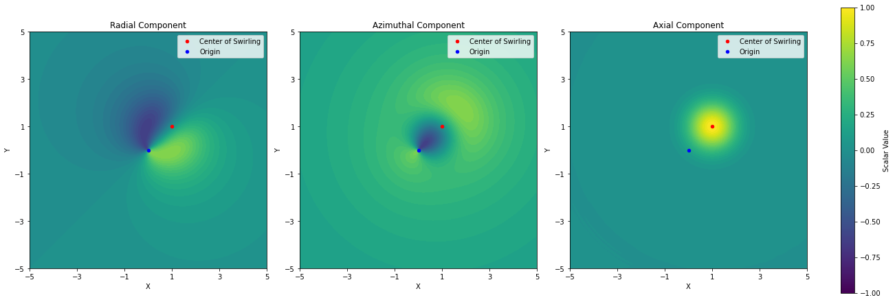
In this tutorial, we consider a off-centered swirling vector field with a Gaussian jet component including an intensity adjustment parameter \( q ( \ne 0 ) \):

\[\mathbf{V}(r', \phi', z) = \frac{1 - \exp(-r'^2)}{r'} \hat{\mathbf{e}}_{\phi'} + \frac{\exp (-r'^2)}{q} \hat{\mathbf{e}}_z,\]

where \( (r’, \phi’) \) is translated polar coordinate parameters centered at a centerline \( (r, \phi) = (\sqrt{2}, \pi /4) \), or equivalently, \( (x, y) = (1, 1) \). We fix \( q \) to 1. Using the analytical derivation of \( \psi \) and \( \chi \) (see above), these scalars can be obtained as follows:

\[\psi = -\left( \nabla_\perp^2 \right)^{-1} \left[ 2 \exp (- (r \cos \phi - 1 )^2 - ( r \sin \phi - 1 )^2 ) \right],\] \[\chi = -\left( \nabla_\perp^2 \right)^{-1} \left[ \exp (- (r \cos \phi - 1 )^2 - ( r \sin \phi - 1 )^2 ) \right],\]

because

\[V_z (r) = \exp (- (r \cos \phi - 1 )^2 - ( r \sin \phi - 1 )^2 )\]

and

\[(\nabla \times \mathbf{V})_z (r) = 2\exp (- (r \cos \phi - 1 )^2 - ( r \sin \phi - 1 )^2 ) .\]

Computational generation steps of \( \psi \) and \( \chi \), founded upon the above analytic formula, is described in a program-dependent subroutine qvort_dist() of the current tutorial program in [root_dir]/src/apps/vecfld_reconstruction.f90 and curious users may refer to it. The vector field \( \mathbf{V} \), if interpreted as a flow velocity field, is often called the \(q\)-vortex model, a dimensionless representation of either Batchelor or Lamb-Oseen vortex model.

Reconstruct a Vector Field from Toroidal and Poloidal Scalars

Before running the tutorial program, let’s set up the input parameters:

#! bash
# Run this cell will automatically update the input parameter setup in input_tutorial.params. Otherwise, you can manually create this file using nano, vim, etc.
cd ../ # Navigate to the root directory
cat > input_tutorial.params << EOL
!!! COMPUTATIONAL DOMAIN INFO !!!
# ---------- NR ----------- NP ----------- NZ ----------------------------------
            200            128              8    
# ------ NRCHOP ------- NPCHOP ------- NZCHOP ----------------------------------
            200             65              5    
# --------- ELL --------- ZLEN ------ ZLENxPI ---(IF ZLENxPI==T, ZLEN=ZLEN*PI)--
           5.D0           2.D0              T
#
!!! TIME STEPPING INFO !!!
# ---------- DT ----------- TI --------- TOTT ----------- NI --------- TOTN ----
          1.D-1           0.D0           1.D2              0           1000
#
!!! FIELD PROPERTY INFO !!!
# -------- VISC ----- HYPERPOW ---- HYPERVISC ----------------------------------
          1.D-3              0           0.D0
#
!!! FIELD SAVE INFO !!!
# --------------------- FLDDIR -------------------------------------------------
                  ./output/fld
# ---- ISFLDSAV -- FLDSAVINTVL ---(IF ISFLDSAV!=T, FIELDS ARE NOT SAVED)--------
              T            100
#
!!! DATA LOGGING INFO !!!
# --------------------- LOGDIR -------------------------------------------------
                  ./output/dat
# ---- ISLOGSAV -- LOGSAVINTVL ---(IF ISLOGSAV!=T, LOGS ARE NOT GENERATED)------
              T             10
/* ------------------------------ END OF INPUT ------------------------------ */
EOL

Since this tutorial does not involve time integration, only the computational domain configuration is relevant in the above input setup. To minimize computation time, the number of collocation points and spectral elements in the \( z \) direction has been significantly reduced. However, for practical time-dependent simulations, the \( z \) direction would require a resolution comparable to that of the polar directions to ensure accuracy.

Once the tutorial program vecfld_reconstruction numerically generates \( \psi \) and \( \chi \), stored in [root_dir]/output/fld/psi000000_FFF and [root_dir]/output/fld/chi000000_FFF, respectively, the program then executes tp2vec(psi, chi, vr, vp, vz, tfm) to reconstruct the three vector components \( V_r \), \(V_\phi \) and \( V_z \) in a cylindrical coordinate system \( (r, \phi, z) \):

#! bash
cd ../ # Navigate to the root directory, assuming the terminal is opened in the default directory ([root_dir]/tutorials/).
# Do program compilation. You will be able to see what actually this Makefile command runs in the output. 
make vecfld_reconstruction

#! bash
cd ../
# Make sure that the previously generated output files are all deleted.
rm -rf output
# get the total number of processors of your system
np=$(nproc) # if your system can access more than 24 processors, set np <= 24.
echo "The system's total number of processors is $np"
# run the program with your system's full multi-core capacity.
mpirun.openmpi -n $np --oversubscribe ./build/bin/vecfld_reconstruction
# # for ifx + IntelMPI
# mpiexec -n $np ./build/bin/vecfld_reconstruction

#! bash
cd ../output/
# See all generated field files
ls ./fld/

In addtion to psi000000_FFF and chi000000_FFF, you will find three new field files containing the vector components: vr000000_PPP, vp000000_PPP, and vz000000_PPP. Let’s visualize these components to ensure they are correctly reconstructed:

#! Python3
import numpy as np
import matplotlib.pyplot as plt
from matplotlib import cm
from matplotlib.colors import Normalize

# Load static data
NR = 200; NP = 128
coords_r = np.loadtxt('../output/dat/coords_r.dat', skiprows=1, max_rows=NR)
coords_p = np.loadtxt('../output/dat/coords_p.dat', skiprows=1, max_rows=NP)

# Define file paths for the three datasets
files = [
    '../output/fld/vr000000_PPP',
    '../output/fld/vp000000_PPP',
    '../output/fld/vz000000_PPP'
]

# Initialize the figure and axes for three subplots
fig, axes = plt.subplots(1, 3, figsize=(18, 6), facecolor='none', constrained_layout=True)

xlim, ylim = 5, 5
norm = Normalize(vmin=-1, vmax=1)
cmap = cm.viridis

# Titles for each subplot
titles = ['Radial Component', 'Azimuthal Component', 'Axial Component']

for idx, ax in enumerate(axes):
    f_val = np.loadtxt(files[idx], skiprows=1, max_rows=NR)
    
    # Generate X, Y, and Z values
    X_d, Y_d, Z_d = [], [], []
    for index, value in np.ndenumerate(f_val[:NR-1, :NP]):
        x = coords_r[index[0]] * np.cos(coords_p[index[1]])
        y = coords_r[index[0]] * np.sin(coords_p[index[1]])
        z = value
        
        if -xlim <= x <= xlim and -ylim <= y <= ylim:
            X_d.append(x)
            Y_d.append(y)
            Z_d.append(z)
    
    # Plot the contour
    contour = ax.tricontourf(
        X_d, Y_d, Z_d, cmap=cmap, norm=norm, levels=np.linspace(-1, 1, 51), extend='both'
    )
    ax.scatter([1.], [1.], c='r', s=20, label='Center of Swirling')
    ax.scatter([0.], [0.], c='b', s=20, label='Origin')
    ax.set_xlim(-xlim, xlim)
    ax.set_ylim(-ylim, ylim)
    ax.set_xticks(np.linspace(-xlim, xlim, 6))
    ax.set_yticks(np.linspace(-ylim, ylim, 6))
    ax.set_xlabel('X')
    ax.set_ylabel('Y')
    ax.set_aspect('equal')
    ax.set_title(titles[idx])
    ax.legend()

# Add a single colorbar for all plots
fig.colorbar(
    cm.ScalarMappable(norm=norm, cmap=cmap),
    ax=axes, orientation='vertical', fraction=0.02, pad=0.04, label='Scalar Value'
)

plt.show()

Curl of a Vector

Using \( \psi \) and \( \chi \) provides a significant advantage in numerically computing the curl of the vector field, \( \nabla \times \mathbf{V} \), with minimal modifications to MLegS code. By taking the curl on both sides of the TP decomposition formula, we derive:

\[\nabla \times \mathbf{V} = \nabla \times \left\{-\nabla^2 \chi \hat{\mathbf{e}}_z \right\} + \nabla \times \left[ \nabla \times \left\{ \psi \hat{\mathbf{e}}_z \right\} \right].\]

What does this formula imply? If the toroidal-poloidal scalar pair \( (\psi, \chi) \) represents \( \mathbf{V} \), then \( (-\nabla^2 \chi, \psi) \) equivalently represents \( \nabla \times \mathbf{V} \). This means the curl can be computed without any explicit vector differentiation, simply by swapping \( \psi \) with \( \nabla^2 \chi \) and \( \chi \) with \( \psi \). In MLegS, the operation can be implemented with an only two-line addition as:

!# Fortran
! ...
call del2(chi, tfm) ! Compute the Laplacian of chi
chi%e = -chi%e ! Negative sign to del2(chi)
call tp2vec(chi, psi, wr, wp, wz, tfm) ! (wr, wp, wz) represents the curl of the vector field
! ...

For those who wish to avoid confusion from manually switching \( \psi \) and \( \chi \), MLegS provides a shorthanded subroutine, tp2curlvec(), to directly compute the curl:

!# Fortran
! ...
! psi, chi: toroidal and poloidal scalars of the vector field, (vr, vp, vz) component-wisely
call tp2curlvec(psi, chi, wr, wp, wz, tfm) ! (wr, wp, wz) stores the curled vector's radial, azimuthal and axial components
! ...

Although tp2curlvec() is not included in the tutorial program, you can replace tp2vec() with tp2curlvec() in the tutorial program code and see that it correctly generates the curl of \( \mathbf{V} \).

---

Project a Vector Field into its Toroidal and Poloidal Components

Now that we have the three vector component information in vr000000_PPP, vp000000_PPP, and vz000000_PPP, let’s convert it back to its toroidal and poloidal scalars and verify that these converted scalars are the same as the original scalars used to reconstruct the vector components. Another tutorial program, tp_project in [root_dir]/src/apps/tp_project.f90, is compiled and run:

#! bash
cd ../ # Navigate to the root directory, assuming the terminal is opened in the default directory ([root_dir]/tutorials/).
# Do program compilation. You will be able to see what actually this Makefile command runs in the output. 
make tp_project

#! bash
cd ../
# get the total number of processors of your system
np=$(nproc) # if your system can access more than 24 processors, set np <= 24.
echo "The system's total number of processors is $np"
# run the program with your system's full multi-core capacity.
mpirun.openmpi -n $np --oversubscribe ./build/bin/tp_project
# # for ifx + IntelMPI
# mpiexec -n $np ./build/bin/tp_project

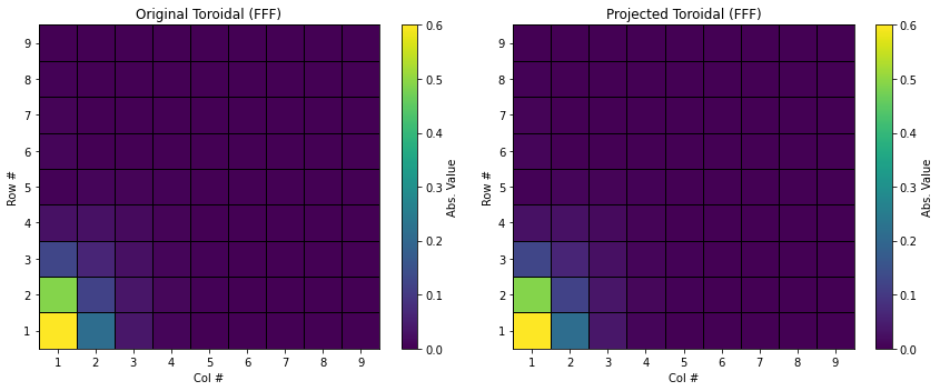
You will see two new field files in the spectral space (FFF): pjpsi000000_FFF and pjchi000000_FFF.

#! bash
cd ../output/
# See all generated field files
ls ./fld/

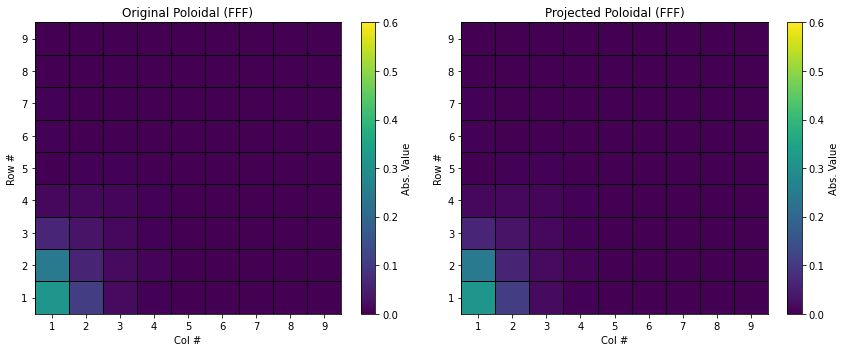
Finally, let’s verify that they are the same as psi000000_FFF and chi000000_FFF, respectively.

#! Python3
def FFF_comparison(data_original_path, data_compared_path, data_original_title, data_compared_title):
    import numpy as np
    import matplotlib.pyplot as plt
    
    # Load MLegS data from files
    NRCHOP = 32; NPCHOP = 25
    data_original = np.loadtxt(data_original_path, skiprows=1, max_rows=NRCHOP)
    data_compared = np.loadtxt(data_compared_path, skiprows=1, max_rows=NRCHOP)
    
    # Compute the absolute values of complex numbers from alternating columns
    # Separate real and imaginary parts and calculate the magnitude (absolute value)
    data_original = np.abs(data_original[:NRCHOP-1, :NPCHOP*2:2] + 1j * data_original[:NRCHOP-1, 1:NPCHOP*2:2])
    data_compared = np.abs(data_compared[:NRCHOP-1, :NPCHOP*2:2] + 1j * data_compared[:NRCHOP-1, 1:NPCHOP*2:2])
    
    # Create a figure with two subplots
    fig, axs = plt.subplots(1, 2, figsize=(12, 5))
    
    # Set tick labels to start from 1
    for i in range(0,2):
        axs[i].set_xticks(np.arange(0,10) + 0.5)
        axs[i].set_xlabel('Col #')
        axs[i].set_xticklabels(np.arange(1,11))
        axs[i].set_yticks(np.arange(0,10) + 0.5)
        axs[i].set_ylabel('Row #')
        axs[i].set_yticklabels(np.arange(1,11))
    
    # Plot original data heatmap
    cax1 = axs[0].pcolormesh(data_original[0:9, 0:9], cmap='viridis', edgecolors='black', vmin=0, vmax=0.6, linewidth=0.5)
    axs[0].set_title(data_original_title)
    fig.colorbar(cax1, ax=axs[0], orientation='vertical', label='Abs. Value')
    
    # Plot compared data heatmap with dividers
    cax2 = axs[1].pcolormesh(data_compared[0:9, 0:9], cmap='viridis', edgecolors='black', vmin=0, vmax=0.6, linewidth=0.5)
    axs[1].set_title(data_compared_title)
    fig.colorbar(cax2, ax=axs[1], orientation='vertical', label='Abs. Value')
    
    # Display the plot
    plt.tight_layout()
    plt.show()

FFF_comparison('../output/fld/psi000000_FFF', '../output/fld/pjpsi000000_FFF', "Original Toroidal (FFF)", "Projected Toroidal (FFF)")

#! Python3
FFF_comparison('../output/fld/chi000000_FFF', '../output/fld/pjchi000000_FFF', "Original Poloidal (FFF)", "Projected Poloidal (FFF)")

vec2tp() for a Non-Solenoidal Vector Field

What happens if the input vector field components vr, vp, and vz do not satisfy the solenoidal field assumption? The answer is straightforward: vec2tp(vr, vp, vz, psi, chi, tfm) will still execute, but only the solenoidal projection of \( \mathbf{V} \) will be retained in terms of \( \psi \) and \( \chi \). Any gradient field component of \( \mathbf{V} \) will be discarded.

According to the Helmholtz decomposition theorem, any generic (smooth) vector field \( \mathbf{U} \) can be decomposed as:

\[\mathbf{U} = - \nabla \Phi + \mathbf{V},\]

where \( \Phi \) is the scalar potential of the gradient field of \( \mathbf{U} \), and \( \mathbf{V} \) is the solenoidal component of \( \mathbf{U} \). If the vector field is provided component-wise as ur, up, and uz, applying vec2tp() followed by tp2vec() will result in only the solenoidal portion of the field being reconstructed as ur_sol, up_sol, and uz_sol:

!# Fortran
! ...
call vec2tp(ur, up, uz, psi, chi, tfm) ! (psi, chi) contains only the solenoidal portion of U
call tp2vec(psi, chi, ur_sol, up_sol, uz_sol, tfm) ! (ur_sol, up_sol, uz_sol) represents the solenoidal portion of U
ur_gra%e = ur%e - ur_sol%e ! The residual fields (u*_gra below) correspond to the gradient field of U, or -∇Φ
up_gra%e = up%e - up_sol%e ! These fields can be useful to check if the input field U is truly solenoidal:
uz_gra%e = uz%e - uz_sol%e ! if the field is solenoidal, all u*_gra entries must be zero (i.e., u*%e = u*_sol%e).
! ...

The residual fields ur_gra, up_gra, and uz_gra in the above code snippet represent the gradient field \( -\nabla \Phi \) of \( \mathbf{U} \). Perhaps these fields can usefully function as diagnostics to determine whether the input vector field is truly solenoidal.

---

1. Lee, S., & Marcus, P. S. (2023). Linear stability analysis of wake vortices by a spectral method using mapped Legendre functions. Journal of Fluid Mechanics, 967, A2. https://doi.org/10.1017/jfm.2023.455 ↩ ↩²