MLegS Tutorial 04: Spectral Operation

Disclaimer: This MLegS tutorial assumes a Linux or other Unix-based environment that supports bash terminal commands. If you are using Windows, consider installing the Windows Subsystem for Linux (WSL).

In this tutorial, you will apply a differentiation operation to a scalar field in spectral space. Spectral space operations that convert one set of spectral coefficients to another generally provide more accurate results than physical space operations, such as finite differences or other collocation point-based methods. Many differentiation operations can be performed directly within the spectral space, especially for linear operations like the Laplacian \( \nabla^2 \equiv \frac{1}{r} \frac{\partial}{\partial r} \left( r \frac{\partial}{\partial r} \right) + \frac{1}{r^2} \frac{\partial^2}{\partial \phi^2} + \frac{\partial^2}{\partial z^2} \).

MLegS, in its most recent version, provides essential spectral operations commonly used in physical simulations, like the Laplacian \( \nabla^2 \), the radial derivative operator \( r \frac{\partial}{\partial r} \), and the Helmholtz operator \( \nabla^2 + \alpha I \), along with their inverse operations when inversion is feasible. This tutorial explains how these spectral space operations are implemented, using the Laplacian \( \nabla^2 \) and its inverse as examples, so that you can learn the following:

Obtain Laplacian of a Scalar
- Given a scalar field \(s \), its Laplacian, \( \nabla^2 s \), is obtainable via the MLegS built-in subroutine del2().
- The operation does not require the scalar’s physical form and is directly converted in the spectral space.
Get Acquainted with Other Built-In MLegS Spectral Differentiation Operators
- MLegS provides additional differentiation operators, such as the Helmholtz operator \( \nabla^2 + \alpha I \) and the powered Helmholtz operator \( \nabla^{h} + \beta \nabla^2 + \alpha I \) for \( h = 4, 6, 8 \).
- Their mathematical definitions and typical usage in MLegS are presented.

Completing this tutorial will help you apply spectral differentiation operators in MLegS with confidence.

MLegS Tutorial 04: Spectral Operation
1. Obtain Laplacian of a Scalar
2. Get Acquainted with Other Built-In MLegS Spectral Differentiation Operators

Obtain Laplacian of a Scalar

Laplacian

Let’s reuse the scalar field information generated in the previous tutorial (Tutorial 02: Scalar Transformation), stored in [root_dir]/output/dat/scalar_FFF.dat. If you skipped the previous tutorial, don’t worry; the program for this tutorial, laplacian.f90, will create it for you if scalar_FFF.dat does not already exist. However, to comprehend the data type scalar, it is recommended to proceed after completing the previous tutorial.

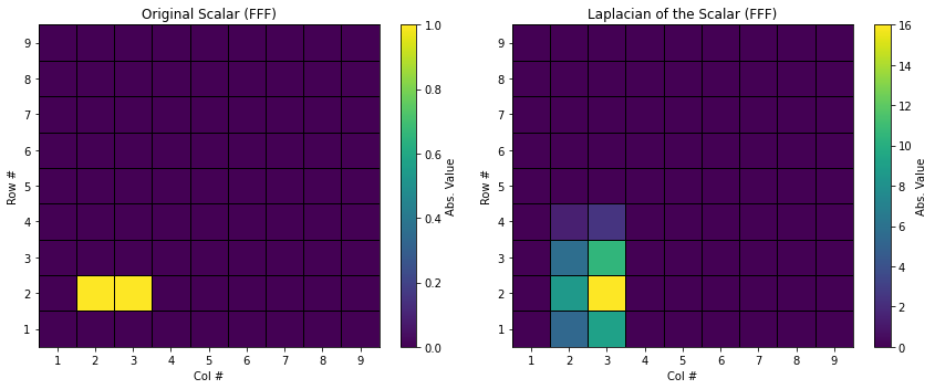
The scalar \( s \), which is 2-dimensional, contains its field data in spectral space form and has only two nonzero spectral coefficients with values of unity: \( s_0^{10} \) and \( s_1^{20} \).

MLegS can quickly compute its Laplacian, \( \nabla^2 s \), directly in spectral space, without requiring any additional computations to transform the scalar to physical space. Given that s is loaded with the spectral coefficient data, you can call the del2() function as follows:

!# Fortran
! ...
call del2(s, tfm)
! ...

The above command replaces the spectral information of s with that of its Laplacian. If you want to keep the original s, declare and initialize another variable of type scalar, say s2, and use:

!# Fortran
! ...
call s2%init(s%glb_sz, s%axis_comm); s2%space = 'FFF'
s2 = s
call del2(s, tfm)
! ...

This way, s2 retains the original scalar data, while s contains the Laplacian of the scalar.

The program laplacian.f90 performs these calculation steps. Run it to obtain the Laplacian data output, which will be saved in [root_dir]/output/dat/scalar_FFF_Laplacian.dat.

#! bash
cd ../ # Navigate to the root directory, assuming the terminal is opened in the default directory ([root_dir]/tutorials/).
# Do program compilation. You will be able to see what actually this Makefile command runs in the output. 
make laplacian

#! bash
cd ../
# get the total number of processors of your system
np=$(nproc) # if your system can access more than 32 processors, set np <= 32.
echo "The system's total number of processors is $np"
# run the program with your system's full multi-core capacity.
mpirun.openmpi -n $np ./build/bin/laplacian
# # for ifx + IntelMPI
# mpiexec -n $np ./build/bin/laplacian

You can visualize how the Laplacian operation in the spectral space alters the distribution of spectral coefficients. Run the following matplotlib code to compare the spectral coefficient distributions between the original scalar and its Laplacian.

#! Python3
# to run this cell, install numpy and matplotlib in your Python3 environment.
def FFF_comparison(data_original_path, data_compared_path, data_original_title, data_compared_title):
    import numpy as np
    import matplotlib.pyplot as plt
    
    # Load MLegS data from files
    NRCHOP = 32; NPCHOP = 25
    data_original = np.loadtxt(data_original_path, skiprows=1, max_rows=NRCHOP)
    data_compared = np.loadtxt(data_compared_path, skiprows=1, max_rows=NRCHOP)
    
    # Compute the absolute values of complex numbers from alternating columns
    # Separate real and imaginary parts and calculate the magnitude (absolute value)
    data_original = np.abs(data_original[:NRCHOP-1, :NPCHOP*2:2] + 1j * data_original[:NRCHOP-1, 1:NPCHOP*2:2])
    data_compared = np.abs(data_compared[:NRCHOP-1, :NPCHOP*2:2] + 1j * data_compared[:NRCHOP-1, 1:NPCHOP*2:2])
    
    # Create a figure with two subplots
    fig, axs = plt.subplots(1, 2, figsize=(12, 5))
    
    # Set tick labels to start from 1
    for i in range(0,2):
        axs[i].set_xticks(np.arange(0,10) + 0.5)
        axs[i].set_xlabel('Col #')
        axs[i].set_xticklabels(np.arange(1,11))
        axs[i].set_yticks(np.arange(0,10) + 0.5)
        axs[i].set_ylabel('Row #')
        axs[i].set_yticklabels(np.arange(1,11))
    
    # Plot original data heatmap
    cax1 = axs[0].pcolormesh(data_original[0:9, 0:9], cmap='viridis', edgecolors='black', linewidth=0.5)
    axs[0].set_title(data_original_title)
    fig.colorbar(cax1, ax=axs[0], orientation='vertical', label='Abs. Value')
    
    # Plot compared data heatmap with dividers
    cax2 = axs[1].pcolormesh(data_compared[0:9, 0:9], cmap='viridis', edgecolors='black', linewidth=0.5)
    axs[1].set_title(data_compared_title)
    fig.colorbar(cax2, ax=axs[1], orientation='vertical', label='Abs. Value')
    
    # Display the plot
    plt.tight_layout()
    plt.show()

FFF_comparison('../output/dat/scalar_FFF.dat', '../output/dat/scalar_FFF_Laplacian.dat', "Original Scalar (FFF)", "Laplacian of the Scalar (FFF)")

png

The tutorial program also provides an additional output file, [root_dir]/output/dat/scalar_PPP_Laplacian, which contains the physical space representation of s. However, note that this spectral-to-physical transformation process is not necessary for actual calculations, as the Laplacian operation can be performed entirely within the spectral form of the scalar.

For instructional purposes, let’s verify that the transformed FFF scalar indeed contains the correct Laplacian by comparing it with the exact analytic form. The scalar field is known to be:

\[s(r,\phi) = 2 \left[ \sqrt{\frac{5}{12}} \cdot \frac{-6 r(r^2 - 1)}{(r^2 + 1 )^2} \cos (\phi) + \sqrt{\frac{7}{240}} \cdot \frac{60 r^2(r^2 - 1)}{(r^2 + 1 )^3} \cos (2 \phi) \right],\]

and therefore its Laplacian is also analytically derivable. For those interested, the exact form of the Laplacian is:

\[\nabla^2 s(r, \phi) = \frac{48 \sqrt{15} r (r^2 - 1) \left( (r^2 + 1) \cos(\phi) - 2 \sqrt{7} r \cos(2 \phi) \right)}{(r^2 + 1)^5}.\]

The matplotlib code snippet below generates a plot that compares the analytic Laplacian with that computed from MLegS.

#! Python3
# to run this cell, install sympy, numpy and matplotlib in your Python3 environment.
import sympy as sp
import numpy as np
import matplotlib.pyplot as plt
import matplotlib.patches as mpatches

# Symbolically declare the analytically exact scalar field
r, phi = sp.symbols('r phi')
laplacian_f = 48*np.math.sqrt(15)*r*(r**2-1)*((r**2+1)*sp.cos(phi)-2*np.math.sqrt(7)*r*sp.cos(2*phi))/(r**2+1)**5

# Generate analytic scalar data for the plot
laplacian_f_num = sp.lambdify((r, phi), laplacian_f)
r_vals = np.linspace(0.01, 5, 500)
phi_vals = np.linspace(0, 2 * np.pi, 64)
R, Phi = np.meshgrid(r_vals, phi_vals)
X = R * np.cos(Phi)
Y = R * np.sin(Phi)
Z = laplacian_f_num(R, Phi)

# Load MLegS data
NR = 32; NP = 48
f_val = np.loadtxt('../output/dat/scalar_PPP_Laplacian.dat', skiprows=1, max_rows=NR)
coords_r = np.loadtxt('../output/dat/coords_r.dat', skiprows=1, max_rows=NR)
coords_p = np.loadtxt('../output/dat/coords_p.dat', skiprows=1, max_rows=NP)
X_d = []; Y_d = []; Z_d = []
for index, value in np.ndenumerate(f_val[:NR-3, :NP]):
    X_d.append(coords_r[index[0]] * np.cos(coords_p[index[1]]))
    Y_d.append(coords_r[index[0]] * np.sin(coords_p[index[1]]))
    Z_d.append(value)

# Create the 3D plot
fig = plt.figure(figsize=(10, 10), facecolor='none')
ax = fig.add_subplot(projection='3d', facecolor='none')

# Plot the surface
surf = ax.plot_surface(X, Y, Z, cmap='viridis', alpha=0.75)

# Create a custom legend entry for the surface
surface_patch = mpatches.Patch(color=plt.cm.viridis(0.5), label='Analytic Laplacian')

# Scatter plot of MLegS data
scatter_plot = ax.scatter(X_d, Y_d, Z_d, s=5, c='b', marker='o', alpha=0.9, label='Spectral Laplacian [MLegS]')

# Set labels and add legend
ax.set_xlabel('X')
ax.set_ylabel('Y')
ax.set_zlabel('Z')
ax.legend(handles=[surface_patch, scatter_plot], labels=['Analytic Laplacian', 'Spectral Laplacian [MLegS]'])

plt.show()

png

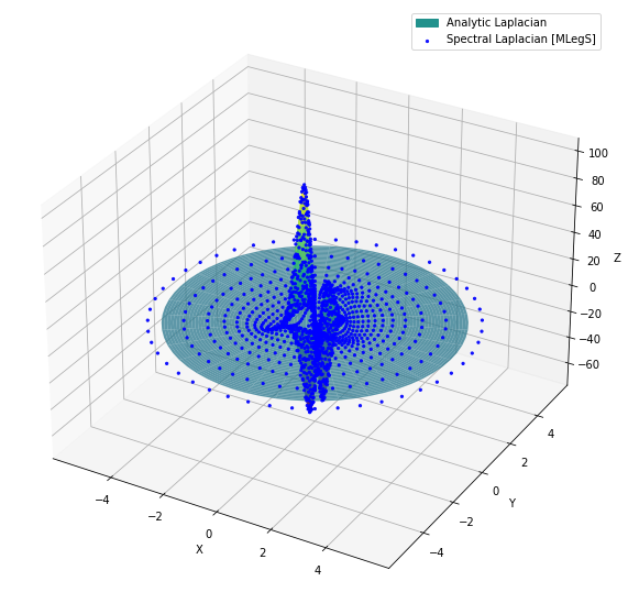
Compare the analytic Laplacian with the discrete points computed from MLegS. It can be confirmed that the spectral operation is perfectly working!

Inverse Laplacian

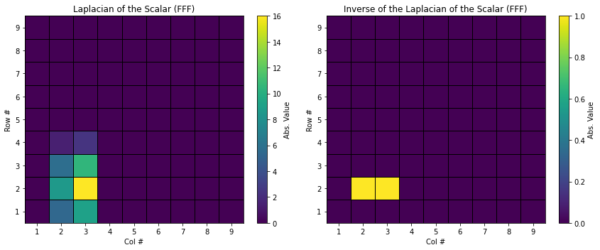
MLegS also provides the inverse Laplacian operation, idel2(), which yields the original scalar field information from its Laplacian. You can compile and run inverse_laplacian.f90, which contains the following commands:

!# Fortran
! ...
call mload(trim(adjustl(LOGDIR)) // 'scalar_FFF_Laplacian.dat', s)
! ...
call idel2(s, tfm)
! ...
call msave(s, trim(adjustl(LOGDIR)) // 'scalar_FFF_from_inv.dat')
! ...

You can check that now s turns into the original scalar field.

#! bash
cd ../ # Navigate to the root directory, assuming the terminal is opened in the default directory ([root_dir]/tutorials/).
# Do program compilation. You will be able to see what actually this Makefile command runs in the output. 
make inverse_laplacian

#! bash
cd ../
# get the total number of processors of your system
np=$(nproc) # if your system can access more than 32 processors, set np <= 32.
echo "The system's total number of processors is $np"
# run the program with your system's full multi-core capacity.
mpirun.openmpi -n $np ./build/bin/inverse_laplacian
# # for ifx + IntelMPI
# mpiexec -n $np ./build/bin/laplacian

#! Python3
FFF_comparison('../output/dat/scalar_FFF_Laplacian.dat', '../output/dat/scalar_FFF_from_inv.dat', "Laplacian of the Scalar (FFF)", "Inverse of the Laplacian of the Scalar (FFF)")

png

How MLegS Treats Constants from Laplacian Inversion

Finding the inverse Laplacian of an arbitrary scalar \( s \) is equivalent to finding a solution \( f \) such that \( \nabla^2 f = s \). The homogeneous form of this problem has two general solutions: \( f_1 = 1 \) and \( f_2 = \ln(r) \), meaning that any scalar field represented as \( f_a = f_p + C_1 + C_2 \ln(r) \) is a solution to \( \nabla^2 f = s \) if \( \nabla^2 f_p = s \). In other words, the inverse Laplacian does not have a unique solution.

MLegS manages these two constants, \( C_1 \) and \( C_2 \), as follows to specify one solution among Laplacian inversions:

Since both \( C_1 \) and \( C_2 \) can be arbitrary, MLegS sets \( C_1 = C_2 \) to reduce the degrees of freedom.
Generally, scalars are expected to decay to zero as \( r \rightarrow \infty \), so \( C_2 \) is typically set to zero (this is why the internal variable %ln in scalar is almost always set to zero). Thus, in most cases, \( C_1 = C_2 = 0 \).
In rare cases where an inverted scalar requires a nonzero logarithmic term with a constant c, the inversion imposes \( C_2 = c \). The idel2() command should then take an additional parameter ln as follows:
```
!# Fortran
! ...
c = some_nonzero_real_value
call idel2(s, tfm, ln=c)
! ...
```

In calculations, the logarithmic term is expressed as \( P_l (r) = \ln((L^2 + r^2) / 2L^2) \), which serves as a proxy for \( \ln(r) \) to maintain analyticity at the origin when the logarithmic term is nonzero. This approach ensures that the scalar behaves as \( O(\ln(r)) \) as \( r \rightarrow \infty \), while \( P_l (r) \) asymptotically matches this behavior without disrupting analyticity at the origin. See Matsushima & Marcus (1997)¹ if one wants to find more details.

If you want to modify the constant field \( C_1 \), simply adjust the value corresponding to \( s_0^{00} \) in the scalar \( s \). This entry, typically located in Row 1, Column 1 of the master processor (proc 0), serves as the coefficient of \( P_{L_0}^{0} (r) \), which by definition is equal to 1 everywhere.

Get Acquainted with Other Built-In MLegS Spectral Differentiation Operators

Scaled 2D Laplacian \( (1-x)^{-2} \nabla_\perp^2 \)

Using the fact that \( P_{L_n}^m (r) \) satisfies the Sturm-Liouville equation:

\[\frac{d}{dr} \left[ r \frac{d}{dr} P_{L_n}^m (r) \right] - \frac{m^2}{r} P_{L_n}^m (r) + \frac{4n(n+1)L^2 r}{(L^2 + r^2)^2} P_{L_n}^m (r) = 0,\]

it is possible to derive the following equality for any \( n \) and \( m \):

\[\left(\frac{L^2 + r^2}{2 L^2}\right)^2 \cdot \left[ \frac{1}{r} \frac{d}{dr} \left[ r \frac{d}{dr} P_{L_n}^m (r) \right] - \frac{m^2}{r^2} P_{L_n}^m (r) \right] = - \frac{n(n+1)}{L^2} P_{L_n}^m (r).\]

Thus, applying the left-hand side differentiation operator with the algebraic multiplication \( \left[ (L^2 + r^2)/(2 L^2)\right]^2 \) to \( P_{L_n}^m (r) \) reduces to a simple multiplication by the factor \( -n(n+1)/L^2 \).

Since \( x \equiv (r^2 - L^2)/(r^2 + L^2) \), it follows that \( 1-x = (2L^2) / (r^2 + L^2 ) \). Consequently, the left-hand side operation can be expressed as:

\[(1-x)^{-2} \nabla_\perp^2 \equiv \left(\frac{L^2 + r^2}{2 L^2}\right)^2 \cdot \left[ \frac{1}{r} \frac{\partial}{\partial r} \left( r \frac{\partial}{\partial r} \right) + \frac{1}{r^2} \frac{\partial^2}{\partial \phi^2} \right].\]

Note that \( \nabla_\perp^2 \) indicates \( \frac{1}{r} \frac{\partial}{\partial r} \left( r \frac{\partial}{\partial r} \right) + \frac{1}{r^2} \frac{\partial^2}{\partial \phi^2} \), which is the 2-dimensional Laplacian that only lacks the derivative in \( z \).

This operation is performed via delsqp() in MLegS:

!# Fortran
call delsqp(s, tfm) ! corresponding inversion operation is idelsqp(s, tfm)

2D Laplacian \( \nabla_\perp^2 \)

2D Laplacian of a scalar can be performed as a spectral space operation:

\[\nabla_\perp^2 \equiv \frac{1}{r} \frac{\partial}{\partial r} \left( r \frac{\partial}{\partial r} \right) + \frac{1}{r^2} \frac{\partial^2}{\partial \phi^2}\]

This operation is performed via del2h() in MLegS:

!# Fortran
call del2h(s, tfm)

Radial Derivative \( rD_r \)

Radial derivative of a scalar with the multiplication of \( r \) can be performed as a spectral space operation:

\[rD_r \equiv r \frac{\partial}{\partial r}\]

This operation is performed via xxdx() in MLegS:

!# Fortran
call xxdx(s, tfm)

Helmholtz \( H \)

Helmholtz of a scalar \( s \) adds the \(\alpha\)-fold of \( s\) to its Laplacian, \( \nabla^2 s \):

\[H \equiv \nabla^2 + \alpha I\]

This operation is performed via helm() in MLegS:

!# Fortran
call helm(s, alpha, tfm) ! corresp. inversion operation is ihelm(s, alpha, tfm)

Powered Helmholtz \( H_p \)

Powered Helmholtz of a scalar \( s \) gets the sum of the \(\alpha\)-fold of \( s\), \(\beta\)-fold of its Laplacian, \( \nabla^2 s \), and \( \nabla^p s \) for \( p = 4, 6 \) or \( 8 \).

\[H_p \equiv \nabla^p + \beta \nabla^2 + \alpha I\]