MLegS Tutorial 05: Time Integration

Disclaimer: This MLegS tutorial assumes a Linux or other Unix-based environment that supports bash terminal commands. If you are using Windows, consider installing the Windows Subsystem for Linux (WSL).

This tutorial introduces the built-in time integration schemes available in MLegS. Currently, MLegS supports first-order and second-order time integration methods, providing global accuracy of \( O(\Delta t) \) and \( O(\Delta t^2) \), respectively, depending on the time-stepping interval \( \Delta t \).

All time integration schemes in MLegS are either fully explicit (fefe() and abab()) or semi-implicit (febe() and abcn()). The semi-implicit schemes help address the numerical stiffness posed by the diffusion term by treating it separately from the advection term, balancing numerical stability and computational efficiency.

In this tutorial, you will:

Apply the First-Order Time Integration Scheme
- You will learn how to use the first-order time integration scheme to simulate temporal evolution based on governing equations and initial conditions, based on the semi-implicit febe() scheme.
Apply the Second-Order Time Integration Scheme
- You will understand how the second-order scheme requires additional field information after one time step at \( t = \Delta t \) and how Richardson extrapolation can be used for bootstrapping, based on the semi-implicit abcn() scheme.

Completing this tutorial will enable you to implement MLegS’s time integration schemes effectively for your simulations.

MLegS Tutorial 05: Time Integration

Tutorial Problem

Description

In this tutorial, we will solve a simple problem with a known exact solution, allowing us to assess the numerical accuracy of the results. The problem involves the temporal evolution of a 2-dimensional axissymmetric vortex, modeled as a Lamb-Oseen vortex, under non-zero viscous dissipation and assuming incompressible flow. The quantity of interest is vorticity, denoted by \( \omega \), with the following initial condition:

\[\omega (r, t=0) = \frac{1}{2\pi} \exp \left(-\frac{r^2}{2}\right),\]

which is non-dimensionalized by scaling the total circulation (\( \Gamma \equiv \int \int \omega \, dS \)) to unity. The governing equation for this problem is the vorticity equation:

\[\frac{\partial \omega}{\partial t} = {\rm{VISC}} \cdot \nabla^2 \omega,\]

where \( {\rm{VISC}} \) is the diffusion coefficient, representing the inverse of the Reynolds number (\( \Gamma / \nu \)) for the vortex motion.

Due to the axisymmetry of the base flow, the advection term (\( u_\phi \cdot \partial \omega / \partial \phi \)) is zero, reducing the governing equation to the scalar diffusion equation. The exact solution for \( \omega(r, t) \) is:

\[\omega(r, t) = \frac{1}{2 \pi \left(1 + 2 \cdot {\rm{VISC}} \cdot t\right)} \exp \left(-\frac{r^2}{2 \left(1 + 2 \cdot {\rm{VISC}} \cdot t\right)}\right).\]

Simulation Setup

For more drastic change in the vorticity in a short run, we set \( {\rm{VISC}} = 0.1 \) (i.e., \( {\rm{Re}} = 10 \) and see the evolution of the vortex up to \( t = 10 \), with a time stepping interval of \( \Delta t = 0.2 \) first. Creating a new input configuration file input_tutorial.params, let’s set up the input parameters as following:

#! bash
# Run this cell will automatically update the input parameter setup in input_tutorial.params. Otherwise, you can manually create this file using nano, vim, etc.
cd ../ # Navigate to the root directory
cat > input_tutorial.params << EOL
!!! COMPUTATIONAL DOMAIN INFO !!!
# ---------- NR ----------- NP ----------- NZ ----------------------------------
             32             48              1    
# ------ NRCHOP ------- NPCHOP ------- NZCHOP ----------------------------------
             32             25              1    
# --------- ELL --------- ZLEN ------ ZLENxPI ---(IF ZLENxPI==T, ZLEN=ZLEN*PI)--
           1.D0           1.D0              F
#
!!! TIME STEPPING INFO !!!
# ---------- DT ----------- TI --------- TOTT ----------- NI --------- TOTN ----
          2.D-1           0.D0           1.D1              0             50
#
!!! FIELD PROPERTY INFO !!!
# -------- VISC ----- HYPERPOW ---- HYPERVISC ----------------------------------
          1.D-1              0           0.D0
#
!!! FIELD SAVE INFO !!!
# --------------------- FLDDIR -------------------------------------------------
                  ./output/fld
# ---- ISFLDSAV -- FLDSAVINTVL ---(IF ISFLDSAV!=T, FIELDS ARE NOT SAVED)--------
              T             50
#
!!! DATA LOGGING INFO !!!
# --------------------- LOGDIR -------------------------------------------------
                  ./output/dat
# ---- ISLOGSAV -- LOGSAVINTVL ---(IF ISLOGSAV!=T, LOGS ARE NOT GENERATED)------
              T              1
/* ------------------------------ END OF INPUT ------------------------------ */
EOL

Apply the First-Order Time Integration Scheme

The tutorial program, time_integration_first is written in [root_dir]/src/apps/time_integration_first.f90. Let’s compile and run this program first.

#! bash
cd ../ # Navigate to the root directory, assuming the terminal is opened in the default directory ([root_dir]/tutorials/).
# Do program compilation. You will be able to see what actually this Makefile command runs in the output. 
make time_integration_first

#! bash
cd ../
# Make sure that the previous output files, from time_integration_first are all deleted.
rm -rf output
# get the total number of processors of your system
np=$(nproc) # if your system can access more than 24 processors, set np <= 24.
echo "The system's total number of processors is $np"
# run the program with your system's full multi-core capacity.
mpirun.openmpi -n $np --oversubscribe ./build/bin/time_integration_first
# # for ifx + IntelMPI
# mpiexec -n $np ./build/bin/time_integration_first

Check that the program generates two field data, sfld000000_PPP at \( t = 0 \) and sfld000050_PPP at \( t = 1 \), all computed with \( \Delta t = 0.2 \), and three log data of the scalar value at origin in terms of time, sval_origin_dt2e-1.dat, sval_origin_dt4e-1.dat and sval_origin_dt1e-0.dat, each computed with varying time stepping intervals of \( \Delta t = 0.2 \), \( \Delta t = 0.4 \) and \( \Delta t = 1.0 \), respectively.

#! bash
cd ../output/
# See all generated fields and data
ls ./fld/ ./dat/

Forward Euler-Backward Euler Time Integration

What does the tutorial program do? It advances the vorticity scalar field w using the semi-implicit Forward Euler-Backward Euler (FE-BE) scheme via MLegS’s built-in febe() subroutine. In the main iterative section of the program, the time-stepping is implemented as follows:

!# Fortran
! ...
!> Run the first-order time stepping
call febe(w, nlw, dt, tfm) ! Forward Euler - Backward Euler time integration by dt
! ...

By running febe(), the field w is advanced by one time step. Since nlw represents the problem-specific non-linear term, it must be updated separately after each time step.

The febe() subroutine assumes a time-dependent differential equation of the form:

\[\frac{\partial w(r,\phi,z,t)}{\partial t} = \underbrace{\mathfrak{A}(w(r,\phi,z,t))}_{\text{Non-stiff (e.g., advection)}} + \underbrace{\mathfrak{L}(w(r,\phi,z,t))}_{\text{Stiff (e.g., diffusion)}},\]

where

\[\mathfrak{L} \equiv \mathrm{VISC} \cdot \nabla^2 - \mathrm{HYPERVISC} \cdot (-\nabla^2)^{\mathrm{HYPERPOW}/2} ,\]

and advances the field w from time step \( k \), denoted as \( w_k \), to the next step \( k+1 \), denoted as \( w_{k+1} \), using the following discretization:

\[\displaylines{ w_{k + 1/2} = w_{k} + \Delta t \cdot \mathfrak{A}(w_{k}) \quad \text{(explicit half-step)} \\ w_{k+1} = w_{k + 1/2} + \Delta t \cdot \mathfrak{L}(w_{k+1}) \quad \text{(implicit half-step)}. }\]

In this tutorial, \( \mathfrak{A} = 0 \) (since there is no advection term due to axisymmetry), and \( \mathfrak{L} = \mathrm{VISC} \cdot \nabla^2 \) (no hyperdiffusion). The FE-BE scheme ensures first-order global accuracy in time.

If you somehow need to handle both stiff and non-stiff terms explicitly, you can use the fefe() subroutine, called the FE-FE scheme, which replaces the implicit backward Euler step with a forward Euler step for the stiff term. While fefe() may avoid additional computing time for implicit calculations, it is highly sensitive to numerical instabilities and often leads to divergence (numerical explosion) early in the simulation.

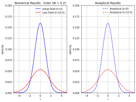
Validation

To validate the numerical results, we compare the computed vorticity fields to their analytical solutions. The following Python code generates plots of the vorticity \( \omega(r) \) at \( t = 0 \) and \( t = 10 \) as functions of the radial coordinate \( r \):

#! Python3
# to run this cell, install numpy and matplotlib in your Python3 environment.
import numpy as np
import matplotlib.pyplot as plt

# Load static data
NR = 32; NP = 48
coords_r = np.loadtxt('../output/dat/coords_r.dat', skiprows=1, max_rows=NR)
coords_p = np.loadtxt('../output/dat/coords_p.dat', skiprows=1, max_rows=NP)

# Load initial and last field data
initial_field = np.loadtxt('../output/fld/sfld000000_PPP', skiprows=1, max_rows=NR)
last_field = np.loadtxt('../output/fld/sfld000050_PPP', skiprows=1, max_rows=NR)

# Analytical solution function
def analytical_solution(y, t, D=0.1):
    r2 = y**2
    return 1 / (2 * np.pi * (1 + 2 * D * t)) * np.exp(-r2 / (2 * (1 + 2 * D * t)))

# Prepare time points for initial and last fields
times = [0, 10.0]  # Initial time t=0 and an example time t=1.0
fields = [("Initial Field", initial_field, times[0], 'b'), 
          ("Last Field", last_field, times[1], 'r')]
xlim = 10  # Limit for the y-axis values

# Initialize the figure
fig, axes = plt.subplots(1, 2, figsize=(8, 6))

# Plot the numerical results
ax_num = axes[0]
for label, field, t, color in fields:
    Y_d, Z_d = [], []
    for index, value in np.ndenumerate(field[:NR-1, :NP]):
        x = coords_r[index[0]] * np.cos(coords_p[index[1]])
        y = coords_r[index[0]] * np.sin(coords_p[index[1]])
        z = value

        if abs(x) <= 1e-6:  # Get the slice at x = 0
            if -xlim <= y <= xlim:
                Y_d.append(y)
                Z_d.append(z)

    # Sort by y for better plotting
    sorted_indices = np.argsort(Y_d)
    Y_d = np.array(Y_d)[sorted_indices]
    Z_d = np.array(Z_d)[sorted_indices]

    ax_num.plot(Y_d, Z_d, label=f"{label} (t={t})", color=color)

ax_num.set_xlim(-5, 5)
ax_num.set_ylim(0, .2)
ax_num.set_xlabel('r')
ax_num.set_ylabel('Vorticity')
ax_num.set_title('Numerical Results - Euler (dt = 0.2)')
ax_num.legend()
ax_num.grid(True)

# Plot the analytical solution
ax_ana = axes[1]
Y_ana = np.linspace(-5, 5, 1000)
for t, color in zip(times, ['b', 'r']):
    Z_ana = analytical_solution(Y_ana, t)
    ax_ana.plot(Y_ana, Z_ana, label=f"Analytical (t={t})", color=color, linestyle='--')

ax_ana.set_xlim(-5, 5)
ax_ana.set_ylim(0, .2)
ax_ana.set_xlabel('r')
ax_ana.set_ylabel('Vorticity')
ax_ana.set_title('Analytical Results')
ax_ana.legend()
ax_ana.grid(True)

# Adjust layout and display the plot
plt.tight_layout()
plt.show()

png

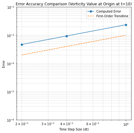
Next, let’s validate the accuracy of the febe() scheme. At \( t = 10 \), the exact vorticity value at the origin is:

\[\omega(r=0, t=10) = \frac{1}{2\pi \cdot (1 + 2 \cdot \mathrm{VISC} \cdot 10)} = \frac{1}{6\pi} \approx 0.05305164769.\]

We can observe the global error trend of the febe() scheme using three different time-stepping intervals: \( \Delta t = 0.2 \), \( \Delta t = 0.4 \), and \( \Delta t = 1.0 \). The error is expected to exhibit a first-order dependency on \( \Delta t \). The following Python code generates the error plot:

#! Python 3
# to run this cell, install sympy, numpy and matplotlib in your Python3 environment.
import numpy as np
import matplotlib.pyplot as plt

# Get the exact vorticity value of w(r=0, t=1)
w_exact = analytical_solution(0.0, 10.0, D=0.1) # Refer to the previous matplotlib cell

# Load the computational results
w_comp_2e_1 = np.loadtxt('../output/dat/sval_origin_dt2e-1.dat', dtype = np.float64)
w_comp_4e_1 = np.loadtxt('../output/dat/sval_origin_dt4e-1.dat', dtype = np.float64)
w_comp_1e_0 = np.loadtxt('../output/dat/sval_origin_dt1e-0.dat', dtype = np.float64)

# Calculate the error
w_err_2e_1 = abs(w_comp_2e_1[-1, -1] - w_exact)
w_err_4e_1 = abs(w_comp_4e_1[-1, -1] - w_exact)
w_err_1e_0 = abs(w_comp_1e_0[-1, -1] - w_exact)

# Time steps
dt = np.array([2e-1, 4e-1, 1e-0])

# Errors
errors = np.array([w_err_2e_1, w_err_4e_1, w_err_1e_0], dtype = np.float64)

# Plot the error comparison
plt.figure(figsize=(6, 6))
plt.loglog(dt, errors, 'o-', label='Computed Error')

# Plot the trendline for first-order accuracy
plt.loglog(dt, 1e-3*dt, '--', label='First-Order Trendline')

# Add labels and legend
plt.xlabel('Time Step Size (dt)')
plt.ylabel('Error')
plt.title('Error Accuracy Comparison (Vorticity Value at Origin at t=10)')
plt.ylim(1e-6, 1e-2)
plt.legend()
plt.grid(True, which='both', linestyle='--', linewidth=0.5)

# Show the plot
plt.tight_layout()
plt.show()

png

Apply the Second-Order Time Integration Scheme

The tutorial program, time_integration_second, is located in [root_dir]/src/apps/time_integration_second.f90. To begin, compile and run the program using the following commands:

#! bash
cd ../ # Navigate to the root directory, assuming the terminal is opened in the default directory ([root_dir]/tutorials/).
# Do program compilation. You will be able to see what actually this Makefile command runs in the output. 
make time_integration_second

#! bash
cd ../
# Make sure that the previous output files, from time_integration_first are all deleted.
rm -rf output
# get the total number of processors of your system
np=$(nproc) # if your system can access more than 24 processors, set np <= 24.
echo "The system's total number of processors is $np"
# run the program with your system's full multi-core capacity.
mpirun.openmpi -n $np --oversubscribe ./build/bin/time_integration_second
# # for ifx + IntelMPI
# mpiexec -n $np ./build/bin/time_integration_second

This second-order time integration program generates the same dataset as the previous tutorial program that uses the first-order time integration scheme.

#! bash
cd ../output/
# See all generated fields and data
ls ./fld/ ./dat/

Adams Bashforth-Crank Nicolson Time Integration

In this program, w is advanced in time using the semi-implicit Adams Bashforth-Crank Nicolson (AB-CN) scheme via MLegS’s built-in abcn() subroutine. The main iterative section of the program implements time-stepping as follows:

! ...
!> Run the second-order time stepping
call abcn(w, w_prev, nlw, nlw_prev, dt, tfm) ! AB-CN time integration by dt
! ...

By running abcn(), the field w is updated one time step forward, and w_prev and nlw_prev are reassigned the field information originally stored in w and nlw, respectively, to account for time advancement. The new time step’s non-linear right-hand side term nlw, which depends on the specific problem being solved, must be updated separately.

Compared to febe(), the abcn() scheme requires field information from the previous time step (w_prev and nlw_prev). For a time-dependent differential equation of the form:

where

\[\mathfrak{L} \equiv \mathrm{VISC} \cdot \nabla^2 - \mathrm{HYPERVISC} \cdot (-\nabla^2)^{\mathrm{HYPERPOW}/2} ,\]

the abcn() subroutine advances the field w from time step \( k \), denoted as \( w_k \), to the next step \( k+1 \), denoted as \( w_{k+1} \), using the following discretization:

\[\displaylines{ w_{k + 1/2} = w_{k} + \Delta t \cdot \left[1.5 \mathfrak{A}(w_{k}) - 0.5 \mathfrak{A}(w_{k-1})\right] \quad \text{(explicit half-step)} \\ w_{k+1} = w_{k + 1/2} + \Delta t \cdot \left[0.5 \mathfrak{L}(w_{k+1}) + 0.5 \mathfrak{L}(w_{k})\right] \quad \text{(implicit half-step)}. }\]

The AB-CN scheme provides second-order global accuracy in time. However, it requires second-order accurate bootstrapping for the field at the first time step (\( t = \Delta t \)). Since the FE-BE scheme only achieves first-order accuracy for \( w_{1} \), Richardson extrapolation is used to enhance the accuracy. The formula for this is:

\[w_{1} = 2 \left. w_{1,~\text{FE-BE}} \right|_{\Delta t / 2} - \left. w_{1,~\text{FE-BE}} \right|_{\Delta t},\]

where the first term on the right-hand side represents the first time step field computed with a time-stepping interval of \( \Delta t / 2 \).

Alternatively, if numerical stability is not a concern, the abab() subroutine (Adams Bashforth-Adams Bashforth scheme) can be used. This replaces the implicit Crank-Nicolson step with an explicit Adams-Bashforth step for the stiff term. However, like fefe(), this approach is generally less stable and is not recommended for systems with significant stiff components.

Validation

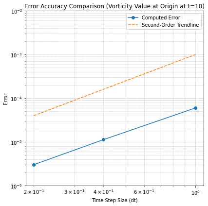
To validate the abcn() scheme, we will compare the numerically computed vorticity fields to their analytical counterparts and verify the scheme’s second-order accuracy in time, as in the previous first-order time integration case.

#! Python3
# to run this cell, install numpy and matplotlib in your Python3 environment.
import numpy as np
import matplotlib.pyplot as plt

# Load static data
NR = 32; NP = 48
coords_r = np.loadtxt('../output/dat/coords_r.dat', skiprows=1, max_rows=NR)
coords_p = np.loadtxt('../output/dat/coords_p.dat', skiprows=1, max_rows=NP)

# Load initial and last field data
initial_field = np.loadtxt('../output/fld/sfld000000_PPP', skiprows=1, max_rows=NR)
last_field = np.loadtxt('../output/fld/sfld000050_PPP', skiprows=1, max_rows=NR)

# Analytical solution function
def analytical_solution(y, t, D=0.1):
    r2 = y**2
    return 1 / (2 * np.pi * (1 + 2 * D * t)) * np.exp(-r2 / (2 * (1 + 2 * D * t)))

# Prepare time points for initial and last fields
times = [0, 10.0]  # Initial time t=0 and an example time t=1.0
fields = [("Initial Field", initial_field, times[0], 'b'), 
          ("Last Field", last_field, times[1], 'r')]
xlim = 10  # Limit for the y-axis values

# Initialize the figure
fig, axes = plt.subplots(1, 2, figsize=(8, 6))

# Plot the numerical results
ax_num = axes[0]
for label, field, t, color in fields:
    Y_d, Z_d = [], []
    for index, value in np.ndenumerate(field[:NR-1, :NP]):
        x = coords_r[index[0]] * np.cos(coords_p[index[1]])
        y = coords_r[index[0]] * np.sin(coords_p[index[1]])
        z = value

        if abs(x) <= 1e-6:  # Get the slice at x = 0
            if -xlim <= y <= xlim:
                Y_d.append(y)
                Z_d.append(z)

    # Sort by y for better plotting
    sorted_indices = np.argsort(Y_d)
    Y_d = np.array(Y_d)[sorted_indices]
    Z_d = np.array(Z_d)[sorted_indices]

    ax_num.plot(Y_d, Z_d, label=f"{label} (t={t})", color=color)

ax_num.set_xlim(-5, 5)
ax_num.set_ylim(0, .2)
ax_num.set_xlabel('r')
ax_num.set_ylabel('Vorticity')
ax_num.set_title('Numerical Results - AB-CN (dt = 0.2)')
ax_num.legend()
ax_num.grid(True)

# Plot the analytical solution
ax_ana = axes[1]
Y_ana = np.linspace(-5, 5, 1000)
for t, color in zip(times, ['b', 'r']):
    Z_ana = analytical_solution(Y_ana, t)
    ax_ana.plot(Y_ana, Z_ana, label=f"Analytical (t={t})", color=color, linestyle='--')

ax_ana.set_xlim(-5, 5)
ax_ana.set_ylim(0, .2)
ax_ana.set_xlabel('r')
ax_ana.set_ylabel('Vorticity')
ax_ana.set_title('Analytical Results')
ax_ana.legend()
ax_ana.grid(True)

# Adjust layout and display the plot
plt.tight_layout()
plt.show()

png

#! Python3
# to run this cell, install sympy, numpy and matplotlib in your Python3 environment.
import numpy as np
import matplotlib.pyplot as plt

# Get the exact vorticity value of w(r=0, t=1)
w_exact = analytical_solution(0.0, 10.0, D=0.1) # Refer to the previous matplotlib cell

# Load the computational results
w_comp_2e_1 = np.loadtxt('../output/dat/sval_origin_dt2e-1.dat', dtype = np.float64)
w_comp_4e_1 = np.loadtxt('../output/dat/sval_origin_dt4e-1.dat', dtype = np.float64)
w_comp_1e_0 = np.loadtxt('../output/dat/sval_origin_dt1e-0.dat', dtype = np.float64)

# Calculate the error
w_err_2e_1 = abs(w_comp_2e_1[-1, -1] - w_exact)
w_err_4e_1 = abs(w_comp_4e_1[-1, -1] - w_exact)
w_err_1e_0 = abs(w_comp_1e_0[-1, -1] - w_exact)

# Time steps
dt = np.array([2e-1, 4e-1, 1e-0])

# Errors
errors = np.array([w_err_2e_1, w_err_4e_1, w_err_1e_0], dtype = np.float64)

# Plot the error comparison
plt.figure(figsize=(6, 6))
plt.loglog(dt, errors, 'o-', label='Computed Error')

# Plot the trendline for first-order accuracy
plt.loglog(dt, 1e-3*dt**2, '--', label='Second-Order Trendline')

# Add labels and legend
plt.xlabel('Time Step Size (dt)')
plt.ylabel('Error')
plt.title('Error Accuracy Comparison (Vorticity Value at Origin at t=10)')
plt.ylim(1e-6, 1e-2)
plt.legend()
plt.grid(True, which='both', linestyle='--', linewidth=0.5)

# Show the plot
plt.tight_layout()
plt.show()

png

MLegS Tutorial 05: Time Integration

Table of Contents

Tutorial Problem

Description

Simulation Setup

Apply the First-Order Time Integration Scheme

Forward Euler-Backward Euler Time Integration

Validation

Apply the Second-Order Time Integration Scheme

Adams Bashforth-Crank Nicolson Time Integration

Validation